The Attention
If you understand attention, you understand transformers. This blog explains the attention mechanism used in modern LLMs. Attention is the core reason transformer-based models like ChatGPT, Gemini, Claude, and Grok work so well. It helps models learn patterns by focusing on the most relevant parts of the input.
Simple Transformer Architecture Diagram
![]()
What is attention?
Attention tells the model where to look. Instead of treating all words equally, it highlights what actually matters for the current prediction. This idea was introduced in Attention Is All You Need (Vaswani et al., 2017).
Attention is not limited to text, the same idea generalizes across audio, images, and video.
Why attention?
Before attention, models like RNNs were slow, sequential, and forgot long-range context. With attention, everything becomes parallel, and the model gets superpowers.
e.g.,
The pilot flies the airplane.
The model learns that pilot -> flies -> airplane are strongly connected.
Scaled Dot-Product Attention block
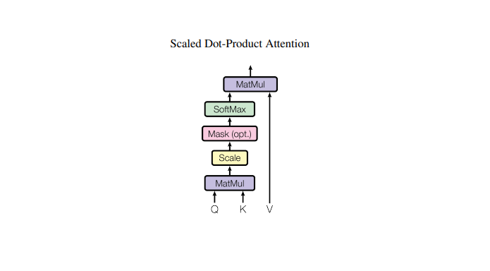
Scaled Dot-Product Attention Formula
This is the entire mechanism in one equation.
Where Q - Query, K - Key, V - Value
Example
Attention is a way for every token to look at all other tokens and decide which ones matter most.
Let's walk through the attention formula with an example step by step. Please refer to the source code here.
We first tokenize the text.
This given sentence is an example text.
2500, 4335, 21872, 382, 448, 4994, 2201, 13
This sentence has 8 tokens. For simplicity, we can reshape it to a tensor of shape (B=2, T=4, C=2). This conversion is needed so the model can learn patterns and assign meaning to each token.
batch (B) - number of independent samples.
seq_len (T) - number of tokens.
hidden_dim ( C) - feature representing each token.
We can read above as two input samples, each sample has 4 tokens, and each token is described by a feature vector of size 2.
After encoding, we get a feature vector from the embedding table. The embedding table stores a vector for each token ID. So, at the start, we assign each token a hidden vector of some defined size (hidden_dim/C) that contains meaning about the tokens, in other words, information. In this case, let's say we are using a hidden dim of size 2 to store information about each token for the sake of simplicity, now the dimension will become (2, 4, 2). These dimensions have names - (batch, seq_len, hidden_dim) or (B, T, C).
Example feature vectors of the first four tokens (random values)
2500  -> [ 1.9269,  1.4873],
4335  -> [ 0.9007, -2.1055],
21872 -> [ 0.6784, -1.2345],
382   -> [-0.0431, -1.6047],
Once we have tokens and their feature vectors, we project these using linear layers to produce Q, K, and V.
C = hidden_dim
query = nn.Linear(C, C)
key = nn.Linear(C, C)
value = nn.Linear(C, C)
# the size of weight matrix present in each vector is CxC

# dim of Q, K, & V ->  (B, T, C)
Q = query(x)
K = key(x)
V = value(x)
print(Q[0])

# first four tokens output of Q
# [ 0.8800, -0.4509], <-- query for 1st token
# [-0.0549, -0.7598], <-- query for 2nd token
# [-0.0850, -0.5294], <-- query for 3rd token
# [-0.5170, -0.3579]  <-- query for 4th token
# same goes for K & V also
This creates three vectors for every token (Q, K, V). These same linear layers are applied across all tokens (shared weights). Once we multiply the input token by these and get unique Q, K, and V for those input tokens.
What it means for a particular token
- Query (Q) - what this token is looking for (what I want).
- Key (K) - how each token presents itself (what tokens offer).
- Value (V) - the information that token carries (information they carry).
Now we compute the dot product between queries and keys by transposing the key across the token dim(1, 2).
# (B, T, C) @ (B, C, T) -> (B, T, T)
attention_scores = (Q @ K.transpose(1, 2))
print(attention_scores[0])

# output
# [ 0.8466, -1.1636, -0.6758, -0.8822],
# [ 1.5116,  0.2629,  0.3584, -0.0411],
# [ 1.0558,  0.2508,  0.2953,  0.0153],
# [ 0.7393,  0.8340,  0.6470,  0.4423]
We multiply all the token's queries by all the token's keys, and this returns a matrix of attention scores. These scores show how much a token shows affinity towards other tokens. Here, each row is a token's details, and each position in a row corresponds to that token's likeness to other tokens. A higher value dot product indicates more focus on this token, lower means less.
e.g., attention_scores[1][2] = 0.3584 shows how much the second token likes the third token.
Once the attention scores are calculated, we normalize these scores. We do this step because large dot products push softmax into saturation and kills gradient flow (softmax saturates), which leads to unstable training. To counteract, we apply 1 / sqrt(d_k).
attention_scores = attention_scores * (K.shape[-1] ** -0.5)
print(attention_scores[0])

# normalized attention scores output
# [ 0.5986, -0.8228, -0.4778, -0.6238],
# [ 1.0688,  0.1859,  0.2534, -0.0291],
# [ 0.7466,  0.1773,  0.2088,  0.0109],
# [ 0.5228,  0.5897,  0.4575,  0.3128]
To make the model predict the next token without cheating, we block future information using a mask. This type of model is called an autoregressive model.
tril = torch.tril(torch.ones(T, T))
attention_scores = attention_scores.masked_fill(tril == 0, float("-inf"))
print(attention_scores[0])

# output after applying the mask
# [ 0.5986,    -inf,    -inf,    -inf], <-- 1st token can only attend to itself
# [ 1.0688,  0.1859,    -inf,    -inf],
# [ 0.7466,  0.1773,  0.2088,    -inf], <-- 3rd token can attend to tokens 1-3
# [ 0.5228,  0.5897,  0.4575,  0.3128]
Each row represents a token, and the first token only attends till 1, the second token first and second, and so on... Future tokens are marked as "-inf," because of that the current token won't be able to take any information, and while predicting the next token, it won't consider the future tokens.
Softmax
Now we will apply softmax to calculate the weighted probability distribution.
atten_wei= F.softmax(attention_scores, dim=-1)
print(atten_wei[0])

# output after applying softmax to attention scores
# [1.0000, 0.0000, 0.0000, 0.0000]
# [0.7074, 0.2926, 0.0000, 0.0000]
# [0.4651, 0.2632, 0.2716, 0.0000] <-- probability distribution for 3rd token
# [0.2620, 0.2802, 0.2455, 0.2124]
The third row tells us how the 3rd token divides its attention across past tokens.
Softmax converts attention scores to a weighted probability distribution that sums up to 1. We use Softmax, which gives us probabilities that either we can utilize to predict the next token or multiply with V to save the contribution in proportion. How much information the current token pulls from others that is in the past or future.
These are important features of softmax.
- Always positive + sums to 1 -> valid probabilities.
- Exponentially emphasizes larger scores -> helps focus attention.
- Smooth and differentiable -> perfect for gradient-based training.
- Attention can spread to all tokens, but softmax and masking often push many weights close to zero.
- Higher probability to higher magnitude and lower to lower.
A table explaining attention scores of third token with softmax probability and how much they will impact value (V).
| Compared token | Attention Scores | softmax probability | Meaning |
|---|---|---|---|
| Token 1 | 0.7466 | 0.465 | highest → token 3 finds token 1 most relevant |
| Token 2 | 0.1773 | 0.263 | lowest → token 3 finds token 2 less relevant |
| Token 3 (itself) | 0.2088 | 0.271 | moderately relevant → some self-attention |
| Token 4 | -inf | 0.000 | masked → future token, ignored |
Now we will apply the weighted sum by doing the dot product between atten_wei and value.
# (B, T, T) @ (B, T, C) -> (B, T, C)
out = atten_wei @ V
print(out[0])

# output after weighted sum
[-0.3642,  0.4548]
[ 0.3499,  0.8945]
[ 0.7720,  1.0779]
[ 1.1964,  1.2087]
The example below shows the weighted sum for the 3rd token's first feature vector in value (V). Since this is the 3rd token, the weight of the fourth is zero, and it won't contribute to the weighted sum for that token.
# 3rd row
print(atten_wei[0,2:3,:])
#[[0.4651, 0.2632, 0.2716, 0.0000]]

# first column of v
print(V[0,:,:1])
# Output
# [[-0.3642],
# [ 2.0765],
# [ 1.4534],
# [ 1.6637]]

# weighted sum for 3rd token's first feature
print(atten_wei[0,2:3,:] @ V[0,:,:1])
#[[0.7720]]
In this scenario, the 4th token has zero contribution because their atten_wei is zero, only the first three tokens have weights. In value, higher probability tokens will contribute more since probability is higher.
Value (V) stores the information that will be mixed based on attention weights. It's storing relevant information for the tokens. Once we calculate the probability of tokens, we do the dot products with value (V) and get the weighted sum. This dot product ensures that high probability will have the higher contribution and low will have lower.
The “out” from attention is fed into feedforward layers, and finally used to predict the next token.
This concludes the attention mechanism calculation that happens inside the transformer block.
Final Thoughts
This is what happens in the attention block.
It takes tokens and their features as an input, passes them through the query, key, and value weight matrix, and then, by using the attention formula, calculates the attention scores and then, by applying softmax, calculates the attention weights, and that helps the model to predict the next token.
Attention is the router of information. Q asks, K answers, and V carries meaning. The model mixes all these pieces to form a richer understanding of each token, and that understanding becomes the next token prediction.
Few other ways to think about the attention mechanism
Weighted lookup Pick the most relevant info from all previous tokens. Ignore useless tokens and amplify important ones.
Soft search engine Each query searches the sequence for what matters.
Dynamic routing Information flows differently for every token.
Content-based addressing Access memory by meaning, not position.
e.g.,
- Connect related words (who is “he” referring to?)
- Pick the right sense of a word (“bank” = money or river)
Basically, attention helps the model focus, remember, and understand better. A neural network learns the patterns in data, and attention improves how well it learns them by directing where to look.
The goal of this blog was to explain how this mechanism works under the hood and develop intuition about it. I wanted to cover the evolution of the attention mechanism also, but then the length of this blog would have been very long, and I wanted to keep this blog short. In Future blogs will cover those topics as well. Use this X post for any comments.
See you in the next blog, and thank you for reading!
Support me here :)
- Follow me on X
- GitHub
- Buy me a coffee.
References
- Attention is all you need (Vaswani et al., 2017)
- Karpathy's GPT from scratch