The Matrix
In this Blog
I've always found matrices more tricky to understand, especially when dealing with high-dimensional tensors. Getting that intuition right is challenging, so I am writing this blog to understand more deeply about matrices/tensors. This blog explores the underlying intuition of the matrix and the operations utilized in training.
What is a matrix?
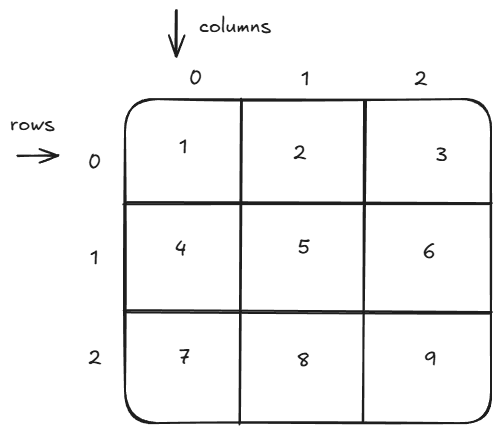
A matrix is a grid of numbers arranged in rows and columns. Think of it like a table where you have rows and columns.
Example:
# in python
[
    [1, 2, 3],
    [4, 5, 6],
    [7, 8, 9],
]

# a matrix with 3 rows and 3 columns
# 0th row - 1, 2, 3
# 0th column - 1, 4, 7
In this case, the matrix has 3 rows and 3 columns. Rows are horizontal, and columns are vertical. Matrix power almost everything in AI. Matrices and their operations are basic Lego blocks of AI. It's basically used in every part of development: pre-training, post-training, and inference. In PyTorch, they are called tensors. I think "tensor" is a cool name, but in this blog I will consider both "matrix" and "tensor" as the same and use them interchangeably. But they are not the same, they are a little bit different. To be more precise,
A matrix is specifically a 2D tensor. Tensors generalize this idea to any number of dimensions. For instance, a scalar (0D), a vector (1D), and a matrix (2D) are all special cases of tensors.
"Matrix" is singular, and "matrices" is plural, and "matrice" is not an English word in mathematics; it's French.
0 dimension - Scalar
# a number e.g.
x = 2
1 Dimension - 1D Tensor - Vector, Array, List
x = [1, 2, 3, 4]
2 Dimension - 2D Tensor - Matrix
x = [
    [1, 2, 3],
    [4, 5, 6],
    [7, 8, 9],
]
# shape - [3, 3]
3 Dimension or more - 3D Tensor or N-D Tensor
x = [
     [
      [1, 2, 3],
      [4, 5, 6],
      [7, 8, 9]
     ]
    ]

# shape- [1, 3, 3]
A very naive way to count the dimension manually is to count the layers of square braces. In the last example, we have 3 layers of square brackets, so it was 3D. And we can go as far as we want with the dimensions, like 4D, 5D...ND.
Multi-dimensional shape intuition
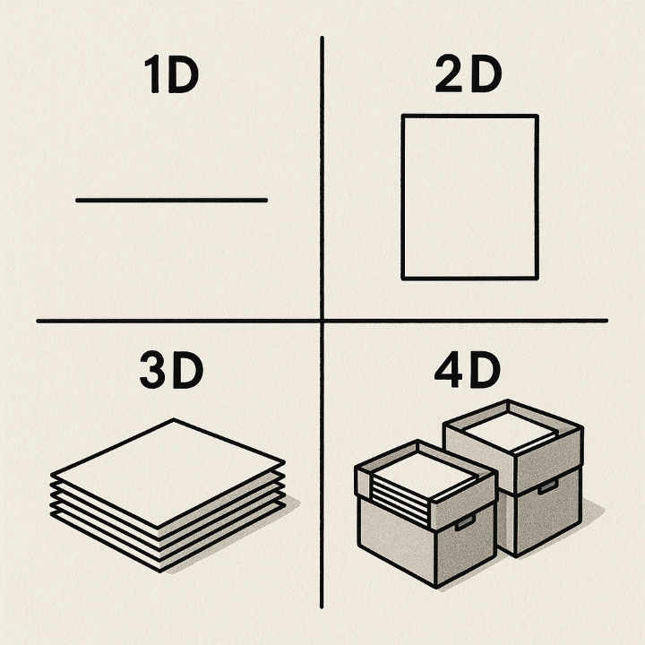
During the model training period we deal with more than 2 dimensions. To get the intuition about higher-dimension tensors, below are a few images.
In this image, 1D is a line on paper, 2D is a single sheet of paper, 3D is many sheets of paper, and 4D is multiple sheets of paper in the boxes.
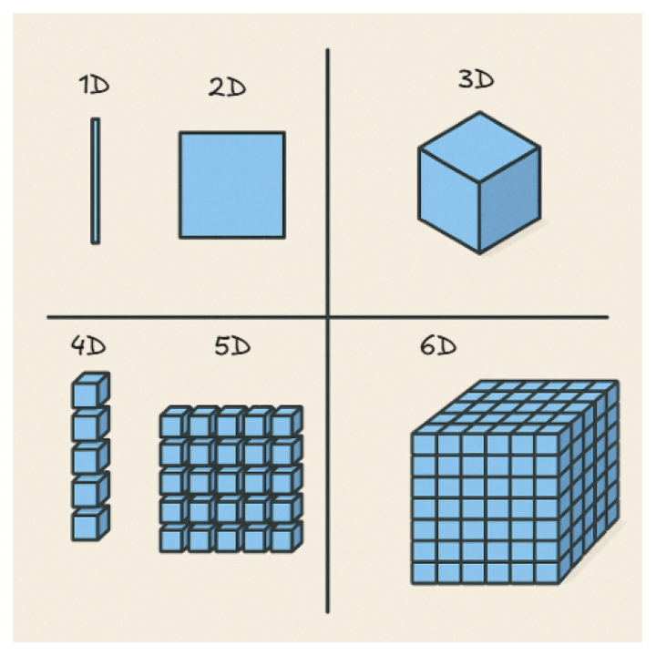
One more way to think about this is to use the cube analogy: a line is 1D, a plane is 2D, a cube is 3D, a stacked cube is 4D, a plane of stacked cubes is 5D, and a cube of stacked cubes is 6D.
Why matrix?
A matrix is simply a structured way to represent data in bulk, especially when you need to perform mathematical operations on it efficiently.
Physics
Matrices represent vectors, transformations, and systems of equations.
Example:
Position of a point in 3D:
r = 2i + 3j + k -> [2, 3, 1]
The above represents the coordinates (x, y, z) of a point in space.
Computer Graphics / Game Design
In graphics, we use matrix operations to move, rotate, scale, or project objects efficiently.
If you want to rotate an object -> multiply by rotation matrix
Scale an object -> multiply by scaling matrix
Translate or project an object -> use homogenous transformation matrix
In simple words these operations let you
- Move an object from one position to another
- Rotate an image clockwise, anticlockwise, or by an angle
- Change size (zoom in/out)
- Apply camera or projection transformations
Data Science
datasets are often represented as matrices.
Rows - samples (observations)
Columns - Features (attributes)
Example:
| Height | weight | age |
|---|---|---|
| 170 | 65 | 25 |
| 160 | 55 | 25 |
as
[
 [170, 65, 25],
 [160, 55, 26]
]
Graph Theory
Adjacency matrix represents the connections between nodes.
A[i][j] = 1 : there is an edge between node i and j, else 0.
Machine Learning
All operations in neural networks primarily involve matrix multiplications and related matrix operations. Inputs, weights, biases, and activations are all represented as matrices/tensors.
Forward pass -> matmuls
Backpropagation -> derivatives on those matrices
Just like matrices transform objects in graphics, they transform data in neural networks.
Images and Videos
- An image is a 2D matrix of pixel values (intensity or color schemes).
- A video is a sequence of image matrices over time (3D or 4D tensors).
Whenever you have structured information that interacts mathematically, represent it as a matrix, because that allows:
- Efficient computation
- Compact representation
- Easy transformation using linear algebra
Example
Once you're able to represent them in a matrix, you can perform many math operations on them. Since this blog's focus is on neural networks, I will pick an LLM input example.
While training LLMs, we use text from the internet or other sources.
# text from tiny shakespeare dataset

We are accounted poor citizens, the patricians good.
What authority surfeits on would relieve us: if they
would yield us but the superfluity, while it were
wholesome, we might guess they relieved us humanely;
but they think we are too dear: the leanness that
afflicts us, the object of our misery, is as an
inventory to particularise their
Now we can't feed these texts directly to the LLMs; they don't process text directly, so we convert it to tokens/integers using a tokenizer. Read my past blog if you want to understand in depth about tokenizers tinybpe.
I used tiktokenizer to covert text to tokens.
# list of tokens for the paragraph
x = [2167, 553, 83982, 12530, 19466, 11, 290, 2506, 2740, 11413, 1899,
 558, 4827, 20515, 1512, 2302, 1348, 402, 1481, 61327, 765, 25, 538,
1023, 198, 83527, 14376, 765, 889, 290, 2539, 32844, 536, 11, 2049, 480,
 1504, 198, 2078, 8795, 747, 11, 581, 3572, 11915, 1023, 91895, 765, 5396,
 1151, 307, 8293, 1023, 2411, 581, 553, 3101, 36203, 25, 290, 505, 934, 436,
 484, 198, 2857, 111894, 765, 11, 290, 2817, 328, 1039, 117394, 11, 382, 472,
 448, 198, 69660, 316, 5024, 1096, 1043]
We can convert the above tokens into matrix with different shapes. To calculate the right shape of the matrix, find out the factor of total number of tokens. In this case I have 84 tokens so factors are - 2 * 2 * 3 * 7. And then we can convert it to any shape that is calculated with these factors like 4 * 3 * 7 or 2 * 6 * 7, 12 * 7, etc. whatever shape you can come up with by multiplying the factors.
Code to convert the list of tokens to some shape of matrix
# Convert list of tokens to torch tensor
x = torch.tensor(x)

# reshape in matrix using valid shapes
x = x.reshape((4, 3, 7))

# or
x = x.reshape((2, 6, 7))
Once the data is converted into tensors, we can perform operations like dot products, additions, and matrix multiplications much faster using GPU and multi-core CPU parallelism. Modern computers can perform trillions of mathematical operations per second, but the challenge is how to use that compute efficiently. A natural idea is: can we train many things at once?
The answer is yes, and this is exactly where matrices (or tensors) come into play. By representing paragraphs of text as numerical tensors (embeddings), we can leverage parallel computation. Each row in the matrix can represent a separate sequence, and multiple batches of such matrices can be processed independently and simultaneously.
This enables vectorized computation, instead of looping over data one sample at a time, the model performs large-scale operations in a single step. As a result, we train models much faster, unlocking a wide range of optimizations that improve performance and scalability.
Here is an example of matrix multiplication using a normal for loop sequential operation and using vectorized CPUs and GPUs with multi-cores.
import torch
import time

# a simple neuron in Neural network
# y = ReLU(wx + b)

# naive Loop
torch.manual_seed(42)
x = torch.randn(1000000)
w = torch.randn(1000000)
b = 0.1

# wx + b
t0 = time.time()
z = b
for i in range(len(x)):
    z += x[i] * w[i]
y = max(0, z)
t1 = time.time()
dt1 = t1 - t0
print(f"Time to calculate Multiplication: {dt1*1000} ms")
# ReLU activation function
print(f"z= {z:.3f}, y= {y:.3f}")

# using vectorized operation
t0 = time.time()
y_vectorized = torch.relu(x @ w + b)
t1 = time.time()
dt2 = t1 - t0
print(f"Time to calculate Multiplication: {dt2*1000} ms")
print(f"y_vectorized= {y_vectorized:.3f}")
print(f"vectorized calculation is {dt1/dt2:.2f}X faster")

### output
# Time to calculate Multiplication: 6897.087097167969 ms
# z= -2214.056, y= 0.000
# Time to calculate Multiplication: 1.0654926300048828 ms
# y_vectorized= 0.000
# vectorized calculation is 6473.14X faster
This example doesn’t reflect the true scale of GPU performance, but it illustrates the idea. Modern GPUs contain thousands of processing cores for example, an RTX 5090-class GPU is expected to have around 21,000 CUDA cores and hundreds of specialized Tensor Cores dedicated to performing matrix multiplications (matmuls). These Tensor Cores, along with NPUs (Neural Processing Units) in newer devices, are optimized specifically for linear algebra operations that power deep learning. The faster they can perform matmuls, the faster and more efficiently a model can train or run locally. Even CPUs today include instruction sets (like AVX-512 or AMX) to accelerate these same tensor operations.
Analogy:
Think of vectorization like commanding an army.
Moving every soldier individually (loop-based operations) is slow and inefficient.
But moving the entire formation at once (vectorized operations) is what GPUs do thousands of “soldiers” moving together in perfect sync.
If the Battle of 300 had been fought on open terrain with the whole formation moving together, it would’ve been over in seconds!
Matrix Operations
This section assumes that you have a basic understanding of Python. For source code and output, refer to the matrix repo. I used PyTorch to perform these operations, a very useful and widely adopted deep learning library.
Convert a normal Python 2D list to a PyTorch tensor.
# A 3 * 3 Matrix
x = [
    [1, 2, 3],
    [4, 5, 6],
    [7, 8, 9],
]
# converting to pytorch tensor -- pytorch represent matrix as a tensor
x = torch.tensor(x)
print(f"shape: {x.shape}")
print(x)
Random
Generating tensors using PyTorch's random method is very useful and used to generate random numbers on demand.
# generate a random 3 * 3 tensor
x = torch.randn(3, 3)
print(x)
Reshape
Transforming 1D tensors into 2D and 3D. As long as the shapes are valid, we can reshape them to any shape.
x = [2167, 553, 83982, 12530, 19466, 11, 290, 2506, 2740, 11413, 1899, 558, 4827, 20515, 1512, 2302, 1348, 402, 1481, 61327, 765, 25, 538, 1023, 198, 83527, 14376, 765, 889, 290, 2539, 32844, 536, 11, 2049, 480, 1504, 198, 2078, 8795, 747, 11, 581, 3572, 11915, 1023, 91895, 765, 5396, 1151, 307, 8293, 1023, 2411, 581, 553, 3101, 36203, 25, 290, 505, 934, 436, 484, 198, 2857, 111894, 765, 11, 290, 2817, 328, 1039, 117394, 11, 382, 472, 448, 198, 69660, 316, 5024, 1096, 1043]
print(f"Length of x: {len(x)}")
x = torch.tensor(x)
print(f"Shape of x: {x.shape}")
x = x.reshape((4, 3, 7))
print(f"Shape of x: {x.shape}")
x = x.reshape((2, 6, 7))
print(f"Shape of x: {x.shape}")
x = x.reshape(12, 7)
print(f"Shape of x: {x.shape}")
Transpose
Convert rows to columns and columns to rows.
# Transpose of matrix
x = torch.randn(2, 3)
print(x.shape)
# transpose the matrix along 0 and 1 dim
x = x.transpose(0, 1)
print(x.shape)
Addition and Substraction
For addition and subtraction we need to have the same shape.
# addition and substraction
x = torch.randn(2, 3)
y = torch.randn(2, 3)
print(x)
print(y)

print("addition: ")
add = x + y
print(add)

print("substraction: ")
sub = x - y
print(sub)

# elementwise mul
print(f"elementwise mul: ")
print(x * y)
Addition and multiplication along axis
x = torch.randint(0, 10, (3, 4))
print(f"x: ")
print(x)

# sum along dimensions
# dim=0 collapse the rows and make one row using sum, along the columns
# if keepdim=True keeps the dimension of actual matrix, if False then return the 1D
z = x.sum(dim=0, keepdim=True)
print(z)

# dim=1 collapse the column and make one column using sum, along the rows
z = x.sum(dim=1)
print(z)

# same goes for multiplication
# dim= 0 collapse the rows and make one row using mul, along the columns
z = x.prod(dim=0, keepdim=True)
print(f"z shape: {z.shape}")
print(z)

# dim= 1 collapse the columns and make one columns using mul, along the rows
z = x.prod(dim=1)
print(z)
Broadcasting
It means applying values to all the values in a given matrix.
We can do broadcasting with compatible shapes.
Rule for broadcasting:
- The dimensions are equal, OR
- One of the dimensions is 1 (it can stretch to match the other size), OR
- One of the tensors has fewer dimensions (the missing dimensions are treated as 1 and stretched).
- broadcast 2 to all elements of matrix.
# broadcasting
x = torch.randint(1, 20, (2, 3))
y = torch.tensor([1, 2, 3])
print(f"x shape: {x.shape}, y shape: {y.shape}")
print(x)
print(y)

# y is added to x in each row
z = x + y
print(z)
# broadcast 2 to all the element of x
print(f"add one element: ")
print(x + 2)
Reduce operation
Sum, average, and max of all the elements in Tensors.
# sum of all elements
x = torch.randint(0, 10, (3, 4))
print(x)
print(f"sum: {x.sum()}")

# multiplication of elements
print(f"multiplicatoin: {torch.prod(x)}")

# mean of all elements
print(f"mean: {torch.mean(x, dtype=torch.float32)}")

# max of all elements
print(f"max: {x.max()}")
Matrix Multiplication (matmul)
# matmuls
B, T = 2, 4
x = torch.randn(B, T)
y = torch.randn(B, T)
# for matmul we need match the shape
# x = (B, T)
# y = (B, T)
# For matmul we need to follow this rule: (a, b) @ (m, n) if b = n
# In this case we need to tranpose the y matrix
# (B, T) @ (T, B) -> (B, B)
z = x @ y.transpose(0, 1)
z
Reshape, Flatten and View
x = torch.randint(1, 20, (3, 4))
print(f" x shape: {x.shape}")

# reshaping
x = x.reshape(4, 3)
print(f" x shape: {x.shape}")

# flattening
x = x.flatten()
print(x.shape)

#similar to reshape but much more memory efficient
x = x.view(2, 6)
print(x.shape)
Tensor Concatenate
# cat
# this operations concatenate tensors along existing direction
# e.g.
a = torch.randint(1, 20, (2, 2))
b = torch.randint(1, 20, (2, 2))
print("a: ")
print(a)
print("b: ")
print(b)
print("concatenate along rows: ")
# concatenate along dim=0 -> rows
out1 = torch.cat((a, b), dim=0)
print(out1.shape)
print(out1)

print("concatenate along columns: ")
# concatenate along dim=1 -> columns
out2 = torch.cat((a, b), dim=1)
print(out2.shape)
print(out2)

# Note:  keep the dimension compatible
Stack
"dim" means = insert a new dimension at position k.
Analogy:
Think of a and b as two photos (2x2 pixels).
dim=0: Put one photo on top of the other → stack of 2 photos.
dim=1: For each row, put a's row and b's row side by side → wider image.
# stack
# stack tensors along new direction
a = torch.randint(1, 20, (2, 2))
b = torch.randint(1, 20, (2, 2))

print(f"a shape: {a.shape}")
print(a)
print(f"b shape: {b.shape}")
print(b)
# stack along new dimension (dim=0)
out1 = torch.stack((a, b), dim=0)
print(f"out1 shape: {out1.shape}")
print(out1)

# stack along new dimension (dim=1)
out2 = torch.stack((a, b), dim=1)
print(f"out2 shape: {out2.shape}")
print(out2)
Indexing and Slicing
# indexing & slicing
x = torch.randint(1, 20, (3, 4))
print(x)
# indexing works like this
# 1D        2D          so on...
#start:end, start:end   so on...
# e.g.
# print first two rows
print(x[:2])
# all rows with last two columns
print(x[:,2:])

# get the element present at 0, 2
print(x[0,2])
Rotate matrix
# rotation of matrix by some theta
angle = 45
theta = math.radians(angle) # convert in radians

# rotation matrix
# this matrix rotates point x by theta
R = torch.tensor([
    [math.cos(theta), -math.sin(theta)],
    [math.sin(theta), math.cos(theta)]
])

# a 2d tensor
# point (x, y)
points = torch.tensor([
    [1.0, 0.0],
    [0.0, 1.0],
    [1.0, 1.0]
])

rot_points = points @ R.T # transpose if points are row wise in point matrix
print(f"rotated points \n {rot_points}")
Lower Traingle, Upper Triangle
# Lower Triangle and Upper triangle
x = torch.randint(1, 10, (3, 3))
print(f"x \n {x}")
lower_traingle = torch.tril(x)
print(f"lower traingle \n {lower_traingle}")

upper_triangle = torch.triu(x)
print(f"upper triangle\n {upper_triangle}")
Identity matrix
It behaves like 1 in matrix -> I * A = A * I = A
# Identity matrix
identity = torch.eye(3)
print(identity)
Masking
While training LLMs, it is used to prevent the model from looking ahead at the future tokens.
# masking
x = torch.tensor([
    [1, 2, 3],
    [4, 5, 6],
    [7, 8, 9]
])

mask = x % 2 == 0  # even numbers
print(mask)
Inverse
We compute a matrix inverse to undo a linear transformation.
# Inverse
# formula = A * A_inv = I

a = torch.tensor([
    [4.0, 7.0],
    [2.0, 6.0]
])
print(f"a \n {a}")

a_inv = torch.linalg.inv(a)
print(f"a_inv \n {a_inv}")

# check
I = a @ a_inv
print(f"a @ a_inv \n {I}")
print(torch.allclose(I.round(decimals=6), torch.eye(2)))
Eigenvalue and Eigenvector
Eigenvector: it's a special direction that doesn't rotate when the matrix acts on it. It only gets stretched or squished.
Eigenvalue: tells how much it's stretched or squished.
# Eigenvalues and Eigenvectors
import torch

a = torch.tensor([
    [2., -1.],
    [-1., 2.]
])

eigvals, eigvecs = torch.linalg.eigh(a)  # 'h' = hermitian (symmetric)
print(eigvals)
print(eigvecs)
Actually, one of the reasons that transformer architecture is famous is because it allows us to do training in parallel that takes advantage of GPUs' parallelism. We only use those matrix operations in training that we can parallelize. Otherwise, those operations will slow down the entire training and will be very expensive.
Summary
The goal of this blog is to give intuition about matrices/tensors and their operations used in LLM training. Treat this blog as notes where you have operations written at one place, kind of like a handbook. I didn't write all the formulas and cover everything, but this has enough that I can use to explain upcoming blogs. I will keep updating this blog as I encounter new operations. Use this X post for comments.
Yes, I did watch "The Matrix" movie before writing this blog. :)
See you in the next blog, and thank you for reading!
Support me here :)
- Follow me on X
- GitHub
- Buy me a coffee.