Build GPT from scratch

24 Feb, 2026

Introduction
Model Architecture
Training Pipeline
Inference
Final Thoughts

Introduction

GPT stands for
Generative - generate something new by predicting the next word/token in sequence.
Pre-trained - first trained on massive datasets like text (mainly), audio & video.
Transformer - neural network architecture used.

AI has always been defined by its most famous application at the time. A decade ago, it was self-driving cars and image or speech recognition. Today, it’s chatbots, agents, and automation. GPT plays a big role in this shift. It predicts the next word in a sequence, and it does it really well. That simple idea enables things like writing essays, answering questions, and generating code. Since we can control computers through language, in theory, models like GPT could handle all tasks humans do on a computer. We’re still far from that level, but we’re moving in that direction. That’s why we’re going to build GPT from scratch.

tinyGPT is not a full chatbot like ChatGPT, Gemini, Claude, or Grok. It only covers the pre-training stage and works purely with text. It learns to generate text similar to the data it’s trained on, inspired by the approach in Improving Language Understanding by Radford et al.

By the end of this blog, we’ll build our own tiny GPT, train it on the Shakespeare dataset, and generate Shakespeare-like text. Check out the tinyGPT repo for the full implementation if you want to run it yourself. We’ll go through the important parts step by step to understand what’s actually happening. Basic knowledge of Python, PyTorch, and matrix multiplication will help you follow along.

GPT Math

Formally, GPT is a language model that assigns a probability to a sequence of tokens.

P (x_{1}, x_{2}, \dots, x_{T}) = \prod_{t = 1}^{T} P (x_{t} ∣ x_{< t})

This comes from the chain rule of probability and is described in the paper A Neural Probabilistic Language Model by Bengio et al. 2003. It states that the probability of an entire sequence can be decomposed into a product of conditional next-token probabilities. In practice, GPT does not predict a full sentence at once. Instead, it learns to predict the next token given all previous tokens.

P (x_{t} ∣ x_{< t})

Training maximizes the log-likelihood.

\log P (x_{1}, \dots, x_{T}) = \sum_{t = 1}^{T} \log P (x_{t} ∣ x_{< t})

This is exactly what the cross-entropy loss computes during training that we will discuss in the training section.

Sample output of the model after being trained on the tiny Shakespeare dataset.

MARCIUS:
Thy bom and that befer Sack!
None as trung, as neque here this dead?

FRICHENRY

WARD IVUMBERLANw:
I thee kne's not uncused,
Threst he good him to heres make:
Have tread? here at wit with flice dists! but afts theme!
Thee? be you distents brialonius
How to the nign alok Yort ming. Turs, m

In order for any ML model to work, we need three things.
Artificial brain - neural network architectures (Transformer, CNN)
How to train - training pipeline (loss, optimizer, training loop, hyperparams)
What to train - data (preparation, token)

Model Architecture

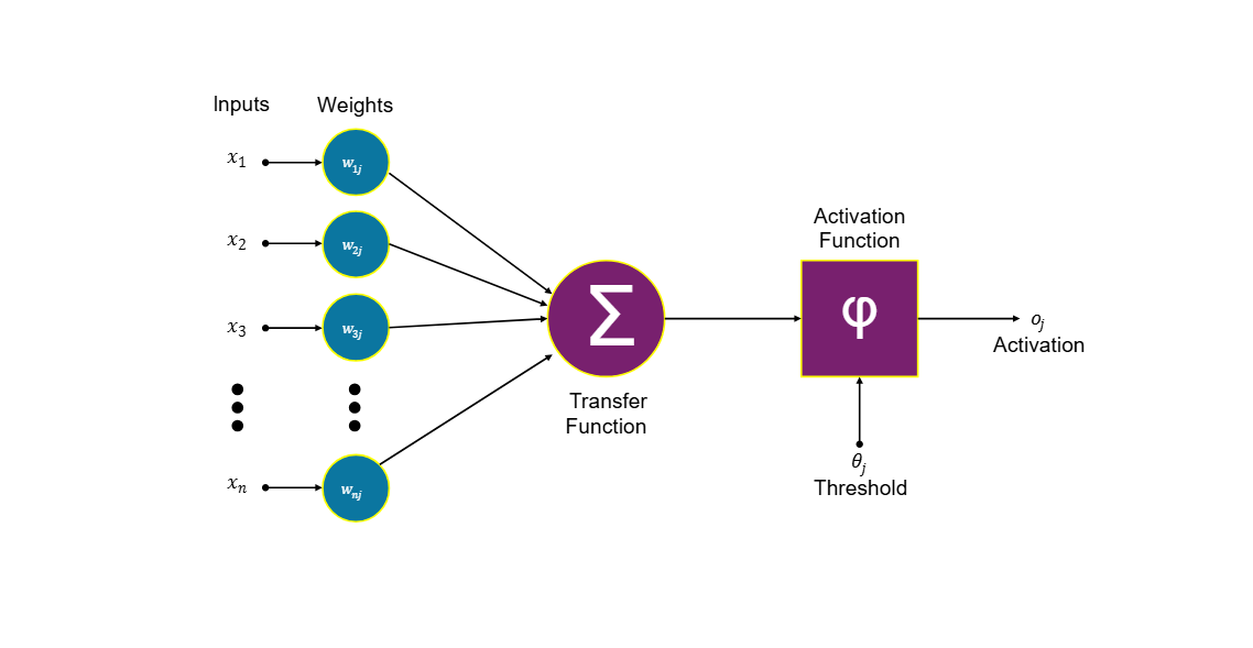
An artificial brain is nothing but a bunch of neural networks (NN) stacked together in some pattern, and these NNs are not the biological ones that are present in our brain. It's a simple mathematical equation. The image below will give you an idea about this.

A single artificial neuron equation

y = max (0, 𝐰^{T} 𝐱 + b)

Python code for single neuron

# Linear equation with Relu non-linearity
# y = x @ W_T + b
# y = max(0, y)

import torch
# seed to fix the random number generation 
torch.seed(42)
# randomly generated 6 numbers
x = torch.randn(6) # input sample (this doesn't change) 
w = torch.randn(6) # weights we change these to improve the output 
y = torch.randn(6) # label
b = 0.1 # bias 

y_hat = torch.relu(x @ w + b)

Here we have a linear equation where w, x, and b are weight, input, and bias, respectively, and y is the output or label. We train and change the weight (w) so our y_hat is as near to y as possible. Once we get the output from wx + b, we pass it through a nonlinear function like Tanh, Sigmoid, ReLU, or many others, in our case, ReLU. This nonlinearity helps the model to learn complex patterns, without it, the whole NN will be a giant linear equation. We are going to nail this part so we can generalize our understanding later.

Mathematical proof for why we need to add nonlinearity.

Layer 1:
h = x*w1 + b1 ----- 1

Layer 2: 
y = h*w2 + b2 ----- 2

then we substitute h in equation 2
y = (x*w1 + b1)w2 + b2
y = x(w1*w2) + (b1*w2 + b2)

so product of w1*w2 -> wn(new weight) and (b1*w2 + b2) -> bn(new bias)
both weights and bias collapsed and it became new weight and bias

y = x*Wn + bn

So, even though there are N number of layers, the whole model will become a giant linear regression. And since this model is linear, it can only represent the straight line or planes, and we can't fit much data to the straight lines. Nonlinearity allows models to bend the space and learn all kinds of patterns in the data. It's all about finding a function that fits the data best. These types of architecture allow the model to fit any data with high accuracy. You can think of it like a statistical machine where you have lots of data and you are writing a math function to explain that data.

Simple Mutiple Layer Perceptron (MLP)

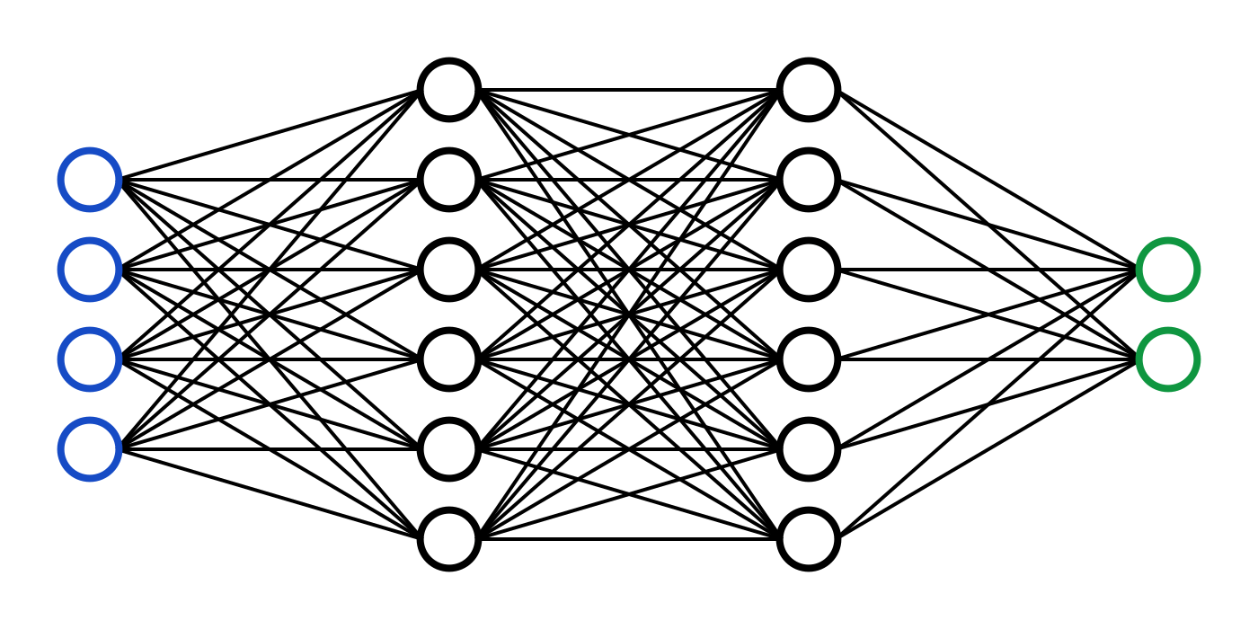
A neuron is the small circle in the MLP. A layer in MLP contains multiple neurons, and there can be n number of layers. So the order is input layer $\to$ hidden layers $\to$ output layer. Each layer takes input from its previous layer and passes output to the next layer. To get the meaningful results from these NN and MLP, we group them in various patterns. TinyGPT and all other chatbots are based on the transformer architecture published in the paper. Attention is all you need, Vaswani et al. The transformer architecture forms the backbone of nearly all modern large language models, Most modern LLMs are architectural refinements and scaling of this architecture.

Transformer Architecture.

Let's start with this architecture. We will start with the main component and slowly work our way down and build the complete architecture. In the decoder-only model we take a token as input and produce the probability of a new token as an output. This architecture has several components.

Input Embeddings - a table to map input tokens to feature vectors.
Positional Embeddings - give the feature vector a sense of the position of tokens in the input.
Masked Multi-Head Attention - make tokens to look at past tokens and derive meaning.
Feedforward Network - gives model space to think and store facts.
Normalization and residual connection - improve overall model performance.
Linear Transformation - project tensor back to vocab size
Softmax Probabilities - probabilities of next tokens

Let's first start with the parent class, where we will code all the components and communication between them, and work our way down and code each component one by one. Refer to the gpt.py code to follow along.

If you see (B, T, C) in the code, that means
B (Batch Dimension) - how many independent input samples we have
T (Time dimension, Block size, Context length, Sequence length) - how far back the model can look/attend tokens while making a prediction.
C (Channel dimension, hidden dimension, Feature vector, n_embd) - how many values to store token information
vocab size - number of words/subwords the model knows about, like a dictionary

These are the model design-related parameters that we have to decide while writing the architecture, these things can't be changed later. And these things affect model size, performance, and cost for training and inference. I will be using PyTorch's inbuilt methods and classes in the example code.

GPT class

device = 'cuda' if torch.cuda.is_available() else 'cpu' # decides where to run the training
block_size = 256
n_embd = 384
n_head = 6
n_layer = 6
dropout = 0.2
class GPT(nn.Module):
    def __init__(self):
        super().__init__()
        # declaration of all the component used in transformer block
        self.token_embedding_table = nn.Embedding(vocab_size, n_embd)
        self.position_embedding_table = nn.Embedding(block_size, n_embd)
        self.blocks = nn.Sequential(*[Block(n_embd, n_head=n_head) for _ in range(n_layer)])
        self.ln_f = nn.LayerNorm(n_embd) 
        self.lm_head = nn.Linear(n_embd, vocab_size)
        self.apply(self._init_weights)
    
    def _init_weights(self, module):
        """
        Initialzing weights before training
        """
        if isinstance(module, nn.Linear):
            torch.nn.init.normal_(module.weight, mean=0.0, std=0.02)
            if module.bias is not None:
                torch.nn.init.zeros_(module.bias)
        elif isinstance(module, nn.Embedding):
           torch.nn.init.normal_(module.weight, mean=0.0, std=0.02)
    
    def forward(self, idx, targets=None):
        # this is how all the component interact with each other in transformer block from start to end

        B, T = idx.shape  # input sequence size

        # embedding table to get the feature vector for input tokens 
        tok_emb = self.token_embedding_table(idx) # (B, T, C)

        # position embedding table to get position related information for each index of the token
        pos_emb = self.position_embedding_table(torch.arange(T, device=device)) # (T, C)

        # adding the token feature and position related information to get the better idea about input sequence
        x = tok_emb + pos_emb # (B, T, C)

        # forwarding the token sequence through all the transformer blocks for attention and Feedforward related action
        x = self.blocks(x) # (B, T, C)

        # normalizing the output generated from blocks
        x = self.ln_f(x) # (B, T, C)

        # calculating the logits by projecting the size to vocab size so every token will have their logits 
        # that will be helpful later to calculate probablities
        logits = self.lm_head(x) # (B, T, vocab_size)

        # calculate loss if this is a training run
        # else only logit calculation for inference
        if targets is None:
            loss = None
        else:
            B, T, C = logits.shape
            logits = logits.view(B*T, C)
            targets = targets.view(B*T)
            loss = F.cross_entropy(logits, targets)

        return logits, loss

The above code is the blueprint as well as the actual code that describes what the components present in the transformer block are. First we convert raw text to tokens to understand how tokenizers tokenize text. Check out my blog tinybpe, which explains tokenizers in depth. Token is what we feed into this GPT forward method. idx is tokens shaped (B, T). If you want to visualize the data &architecture flow from input to output, check out these cool websites bbycropft and Transformer Explainer. I would suggest keeping this open in a different tab for visual reference.

def forward(self, idx, targets=None):

Token Embedding Table

Tokens are the representation of words/subwords in the integer form. Once input text gets converted into tokens (integers) through the tokenizer. We pass those tokens through the token embedding table to get the feature vector for each token. A feature vector is a list of float values that describes features of a token, kind of like a description of the token, e.g., [0.123, 0.124, -1.247] or something like this. This tinyGPT has a feature vector of size n_embd = 384. That means this model takes 384 different float values to describe a token. A different way to think is to consider that a feature vector is a position of a token in 384-dimensional space represented by 384 values. It's not possible in reality, but in the case of the model, it's possible.

e.g., the below image shows how we can interpret a token.

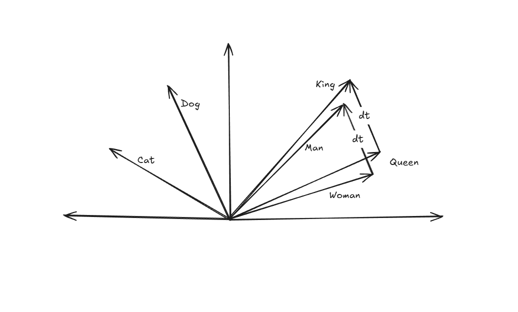
As you can see, the feature vector is pointing to words, similar kinds of words/tokens have similar feature vectors, e.g., "man" and "king" are similar words and are near to each other. Similarly, "woman" and "queen" are similar words, and they are near to each other. The distance vector between king and queen (dt) is the same as the distance vector between man and woman (dt). And there are lots of other interesting things to understand about token relations. I will leave it up to you to investigate more on this if you are interested, and check out this blog as well: Text embedding intro.

Token embedding is a giant table of dimension (vocab_size, n_embd), so based on the token value, it plucks out the row from that table, e.g., token number 69 will pluck out the 69th row from the table. The same goes for other input tokens, and this will form a tensor of dimension (B, T, C). Once we have the feature vector for tokens, now it's time to add position-related information to them.

# declaration in init method of GPT class
self.token_embedding_table = nn.Embedding(vocab_size, n_embd)

# usage under forward method 
tok_emb = self.token_embedding_table(idx) # (B, T, C)

Position Embedding

Position embedding gives the model information about the position of tokens.

Semantic Roles - This adds position-related information to the tokens, e.g.,
The dog bit the man.
The man bit the dog.

Even the frequency of words is the same here, but their order is different. In the first word, "dog" is the actor, and in the second, it is the victim. Without knowing the position of "dog" relative to the verb "bit," the model would treat both sentences as an identical "bag of words." That's where position embedding comes into the picture. It adds the semantic meaning to the words based on their relative orders. Without it, the model will have a hard time getting the context of the sentence right.

Contextual Meaning - position embedding adds the unique vector to each word's representation based on its index. This ensures that the word "the" at position 0 is mathematically distinct from "the" at position 3.

We pass the count of tokens present in the input sequence that is in the range (T). You get the pos embedding vector based on the index from the table. Once we have the position embedding, we add that to the token embedding, and now we have the feature of the tokens and the positional information with us. Both token and position embeddings are learnable parameters, and we train these during training. Modern models often use Rotary Positional Embeddings (RoPE) instead of learned absolute embeddings.

# declaration in init method of GPT class
self.position_embedding_table = nn.Embedding(block_size, n_embd)

# implementation in forward method
pos_emb = self.position_embedding_table(torch.arange(T, device=device)) # (T, C)
# adding the token feature and position related information to get the better idea about input sequence
x = tok_emb + pos_emb # (B, T, C)

LayerNorm - LayerNorm normalizes the feature activations of each token across the embedding dimension. It ensures that the inputs to each layer have a consistent mean and variance, regardless of the batch size. It calculates the mean and variance across all features for a single example. This helps in faster convergence of the model by keeping activation in a healthy range. It allows higher learning rates and helps mitigate the vanishing/exploding gradient problems. Normalization squeezes the feature vector value. We calculate this for each token's feature vector separately, one doesn't depend on the other. LayerNorm is used at multiple places in this architecture, basically at those places where we are about to do the big matmuls, like before calculating self-attention, then before passing through FeedForward, and one after the block. We use the below formula to calculate. First calculate the mean, then the variance, then normalize the feature vector, and then at last we apply beta and gamma as learnable parameters to undo the normalization because we don't want to force every layer to have their value scaled down, we might lose some information because of this. LayerNorm is a tool the model uses rather than a constraint it is trapped by. Normalization stabilizes the number. Gamma ( $γ$ ) and beta ( $β$ ) give back the flexibility to represent complex patterns. Post-norm suffers from gradient instability in deep transformers, which is why GPT models adopt pre-norm.

Mean

μ = \frac{1}{d} \sum_{i = 1}^{d} x_{i}

Variance

σ^{2} = \frac{1}{d} \sum_{i = 1}^{d} (x_{i} - μ)^{2}

Normalize

{\hat{x}}_{i} = \frac{x_{i} - μ}{\sqrt{σ^{2} + ϵ}}

Scale and Shift

y_{i} = γ {\hat{x}}_{i} + β

Pytorch has inbuilt support for LayerNorm

# declaration
self.ln_f = nn.LayerNorm(n_embd)

# normalizing the output generated from blocks
x = self.ln_f(x) # (B, T, C)

When a target/label is present, this means the model is in the training phase, and we need to calculate the loss, and when in the sampling phase, we can skip the loss calculation. We will discuss the loss calculation in the Training section of this blog.

if targets is None:
    loss = None
else:
    B, T, C = logits.shape
    logits = logits.view(B*T, C)
    targets = targets.view(B*T)
    loss = F.cross_entropy(logits, targets)

LM Head

Once the block calculation is done, we feed the output to the lm_head linear layer. This layer projects the feature vector from n_embd to the vocab_size dimension. Later this projection will be used to calculate probabilities of the next token with the help of softmax.

# that will be helpful later in next word prediction
logits = self.lm_head(x) # (B, T, vocab_size)

The Block

Transformer decoder block.

# Forwarding the token sequence through all the transformer blocks for attention and FeedForward 
x = self.blocks(x) # (B, T, C)

Core block has two parts.

Masked multi-head attention
Feedforward Network

These two are the main components of a transformer block, with both having residual connection and normalization through LayerNorm.

class Block(nn.Module):
    def __init__(self, n_embd, n_head):
        super().__init__()
        head_size = n_embd // n_head
        self.sa = MultiHeadAttention(n_head, head_size)
        self.ln1 = nn.LayerNorm(n_embd)
        self.ffwd = FeedForward(n_embd)
        self.ln2 = nn.LayerNorm(n_embd)
    
    def forward(self, x):
        x += self.sa(self.ln1(x)) # (B, T, C)
        x += self.ffwd(self.ln2(x)) # (B, T, C)
        return x

In the above code, we defined the MultiHead attention and Feedforward Network (MLP) segment and made a residual connection between them and also applied normalization through layerNorm.

Residual Connection - Instead of using just the output of self-attention and FeedForward, we add it back to the input y = f(x) + x.

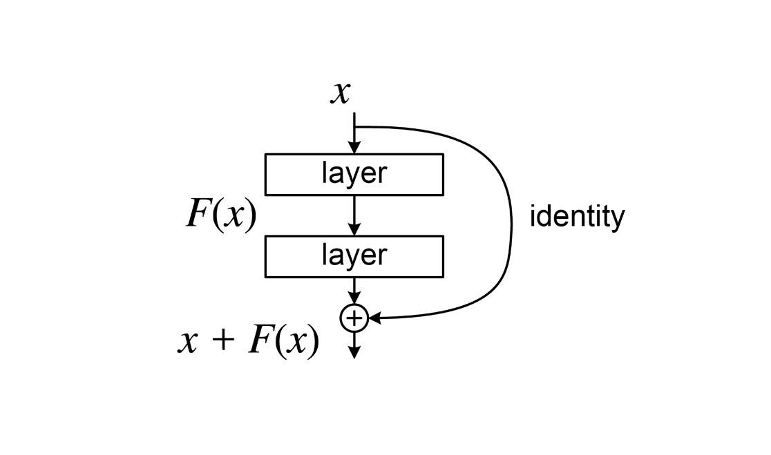
It solves few problems:

Gradient Vanishing - in the deep network, gradients tend to vanish as they pass through many layers during training. Residual connections provide a "highway" for the gradient to bypass the nonlinear layers, ensuring the earlier layers still receive the updates.

Identity Shortcut - if a specific layer is not helpful for the task, the model can simply learn to set the weights of f(x) to zero. This makes layer an identity mapping, letting the information pass through unchanged.

Smoothing the Loss Landscape - without skip connection, the "loss landscape" is extremely jagged and difficult to optimize. Residual connection smooths this surface, making it easier for the model to find the global minimum.

Masked Multi-Head Attention

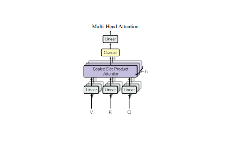
We split an attention head into num_heads times the attention head, forward the input to each head, and concatenate their output.
Why do we do it?

Attention head the reason behind separating the head into multiple smaller heads is that all the heads can be processed in parallel. Since they are being processed in parallel, it allows different heads to learn different concepts, and once concatenated, the model gets the overall view of what the different concepts are being learned and merges that knowledge together.

Dropout is a regularization technique to avoid model overfitting, which means dropout helps the model not to memorize the data but instead to learn the general patterns present in the data. During training, dropout randomly shuts off a fraction of neurons (sets their activation to zero) based on the probability p. This helps a neuron not to depend on certain neurons and forces the neuron to interact with all the surrounding neurons.

Linear Layer project the output from all the heads and concatenate them and pass it through the linear layer. In simple terms, after attention calculation in all the different heads, we merge all the knowledge learned together.

class MultiHeadAttention(nn.Module):
    def __init__(self, num_heads, head_size):
        super().__init__()
        self.heads = nn.ModuleList([Head(head_size) for _ in range(num_heads)])
        self.proj = nn.Linear(num_heads * head_size, n_embd)
        self.dropout = nn.Dropout(dropout)
    
    def forward(self, x):
        out = torch.cat([h(x) for h in self.heads], dim= -1) # concatenate along last dimension
        out = self.dropout(self.proj(out)) # (B, T, C)
        return out

Scaled Dot Product Attention

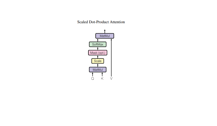
Now we will go through the single attention block and see what's going on inside.

This is the main block of transformer architecture, in other words, this is where all the magic happens the attention block. I have a detailed blog explaining everything about the attention mechanism. The Attention if you want to dig deeper, I would recommend you to read this. Anyway, I will explain the block in brief here so we have the intuition of what is happening here.

What happens inside this block?
In simple words, self-attention enables model to look at the past tokens and derive meaning from them before making a next word prediction.
How? Let's walk it through.
Once we receive the input x, we pass it through three different linear projections: q, k, and v.

These different projections act differently.
Query (q) - what this token is looking for (what I want).
Key (k) - how each token presents itself (what tokens offer).
Value (v) - the information that the token carries (information they carry).

Once we do the projection, we calculate the attention score by doing the dot product between the query and the key. Then we apply scaling factor $1 / \sqrt{d_{k}}$ this prevents the dot-product magnitude from growing too large as dimensions increases. A positive attention score means this token finds the other token more interesting, and a negative value means this token finds that token less interesting. Then we do masking. After we mask, the score means we stop the current token to look into the future, and it can only look in the past. So the first token can look up to the first, the second to the second, and so on. We use a mask with softmax to achieve this.

Now we will apply the weighted sum by doing the dot product between wei and value. Value stores the information that is mixed based on attention weights. It's like storing relevant information for the tokens. The self-attention mechanism has quadratic time and memory complexity O(T²) with respect to sequence length. This is one of the main bottlenecks in scaling transformers to long contexts.

In comments I've mentioned how the tensor weights are transformed before and after the dot product.

import math

class Head(nn.Module):
    def __init__(self, head_size):
        self.query = nn.Linear(n_embd, head_size, bias=False)
        self.key = nn.Linear(n_embd, head_size, bias=False)
        self.value = nn.Linear(n_embd, head_size, bias=False)
        self.register_buffer('tril', torch.tril(torch.ones(block_size, block_size)))
        self.dropout = nn.Dropout(dropout)
    
    def forward(self, x):
        # input of size (batch, tim)
        B, T, C = x.shape

        q = self.query(x) # (B, T, C) -> (B, T, hs)
        k = self.key(x) # (B, T, C) -> (B, T, hs)

        wei = q @ k.transpose(-2, -1) / math.sqrt(k.shape[-1]) # (B, T, hs) @ (B, hs, T) -> (B, T, T)
        # Now mask the wei so it can't attend the future tokens
        wei = wei.masked_fill(self.tril[:T,:T] == 0, float('-inf')) # (B, T, T)
        wei = F.softmax(wei, dim=-1) # (B, T, T)
        wei = self.dropout(wei)
        # perfom the weighted aggregation of the values
        v = self.value(x) # (B, T, c) -> (B, T, hs)
        out = wei @ v # (B, T, T) @ (B, T, hs) -> (B, T, hs)
        return out

Feedforward Network

Once attention is calculated over the tokens, it goes through the FeedForward block, also called the MLP block. While self-attention allows the model to look at other words to gain the context. The FeedForward block is like a knowledge storage for the model, this layer stores the factual knowledge and patterns during training. Think of it as each word taking its newly acquired context from the attention layer and "thinking" about it in isolation. The feedforward network increases model capacity by introducing nonlinearity and expanding representation dimensionality. This layer is made of two linear layers and ReLU (non-linearity) in between. We expanded the linear layer by 4 * n_embd. This allows the model to map the features into higher-dimensional space, where it can learn more complex patterns, and to give more space to the model to think. The expansion by 4 * n_embd is an empirical choice from the transformer paper. While it is not strictly accurate to say the feedforward network alone stores knowledge, empirical studies suggest much of the model’s memorized factual content is localized in MLP layers. Modern transformer implementations often use GELU instead of ReLU for smoother gradients, but I wanted to be consistent with the transformer paper.

class FeedForward(nn.Module):
    def __init__(self, n_embd):
        super().__init__()
        self.net = nn.Sequential(
            nn.Linear(n_embd, 4 * n_embd), 
            nn.ReLU(),
            nn.Linear(4 * n_embd, n_embd),
            nn.Dropout(dropout)
        )

    def forward(self, x):
        return self.net(x)

Training

Our transformer model architecture is ready. Let's start with the training loop. And slowly we will build all the components that are required.

# training loop
for iter in range(max_iters):

    # evaluate the loss after certain iterations 
    if iter % eval_interval == 0 or iter == max_iters - 1:
        losses = estimate_loss()
        print(f"step {iter}: train loss {losses['train']:.4f}, val loss {losses['val']:.4f}")

    # training data
    xb, yb = get_batch('train')

    # evaluate the loss
    logits, loss = model(xb, yb) # forward pass
    optimizer.zero_grad(set_to_none=True) # set gradient to zero
    loss.backward() # calculate the gradient
    optimizer.step() # and update the values of parameter

Char Level Tokenizer

The first thing in the training loop is that we need to get the data. For data, we're going to use the tiny Shakespeare dataset. This file contains works of Shakespeare in text format. We can't feed text directly, in order to train the model with this data, we need to convert these texts to tokens (integer values). So the model can process it and assign it some meaning. Since we have less data, we will use the character-level tokenizer for this, but the character-level tokenizer is not the actual tokenizer used in modern-day LLMs. If you want to understand how tokenizers are used today, check out my blog tinybpe. In a single sentence, a tokenizer converts text to a token (integer value) so the model can process it.

In the code we read the input.txt, filtered out all the unique characters, and sorted them, and in the stoi dict we assigned the unique index to each character and in the itos dict vice versa. Then we have encode and decode, wherein in encode we are taking a string and converting that to a list of tokens, and in decode, vice versa.

# read the file
with open('.tinygpt/data/input.txt', r, encoding='utf-8') as f:
    text = f.read()

chars = sorted(list(set(text)))
vocab_size = len(chars)
stoi = {ch:i for i, ch in enumerate(chars)}
itos = {i:ch for i, ch in enumerate(chars)}
# encoder take a string, and output list of integers
encode = lambda s: [stoi[c] for c in s] 
# decoder: take a list of integers, output a string
decode = lambda l: ''.join([itos[i] for i in l])

Now that our character-level tokenizer is ready. We will split the data into two parts the first will be 'train' and the second for 'val,' as we do in any neural network model.

# Train and test split
data = torch.tensor(encode(text), dtype=torch.long)
n = int(0.9 * len(data))
train_data = data[:n]
val_data = data[n:]

Once the train and val split is done, now we can prep our data. This below method, get_batch, based on the input passed to it, takes the train or val data, generates a list of random integers in between (0, len(data) - block_size), and stacks the x train data and y label. This data loader is very minimal but does the work for a model of this size, here we are not training with a bigger and more versatile dataset.

batch_size = 8
def get_batch(split):
    # generates a small batch of data of inputs x and targets y
    data = train_data if split == 'train' else val_data
    ix = torch.randint(len(data) - block_size, (batch_size,))
    x = torch.stack([data[i:i+block_size] for i in ix])
    y = torch.stack([data[i+1:i+block_size+1] for i in ix])
    x, y = x.to(device), y.to(device)
    return x, y

Now our training data is ready. The next thing in the training loop is to forward the training data and labels through the model.

# model object
model = GPT()
m = model.to(device)
# numbers of parameter in the model
print(sum(p.numel() for p in model.parameters())/1e6, 'M parameters')

When we create an instance of this GPT class, all model weights get initialized with values whose mean is 0.0 and standard deviation (SD) is 0.02. This is also a crucial step, this step ensures that weights are near zero but not actually zero and not some very big value. Research shows that good weight initialization tends to work better in training, and models converge faster than models whose weights are randomly initialized. For example, if all weights started at the same value (like 0), every neuron in a layer would calculate the same output and receive the same gradient update. Neurons would stay synchronized, making the network act like a single neuron. Small random values ensure each neuron learns something different.

Initial Value
Too Large - Gradient explodes, leading to NaN errors.
Too Small - Gradient collapses before reaching the early layers.

A mean of 0.0 centers the data, which helps in stabilizing the search for a global minimum. Std = 0.02 This value was popularized by the original GPT papers. It is a "Goldilocks" number for deep transformers, small enough to prevent explosion but large enough to keep the gradient flowing. Modern models often use Xavier/Kaiming initialization. Starting with bias=0 is common practice.

def _init_weights(self, module):
    """
    Initialzing weights before training
    """
    if isinstance(module, nn.Linear):
        torch.nn.init.normal_(module.weight, mean=0.0, std=0.02)
        if module.bias is not None:
            torch.nn.init.zeros_(module.bias)
    elif isinstance(module, nn.Embedding):
        torch.nn.init.normal_(module.weight, mean=0.0, std=0.02)

We forward the input and label from the model, this is called a forward pass, and we get the logits and loss back.

logits, loss = model(xb, yb) # forward pass

And we keep running this loop long enough till we don't see much progress in this case.

max_iters = 2000
eval_interval = 100

For logging while training runs, we calculate a few things to determine if the model is progressing or not.

if iter % eval_interval == 0 or iter == max_iters - 1:
    losses = estimate_loss()
    print(f"step {iter}: train loss {losses['train']:.4f}, val loss {losses['val']:.4f}")

Forward Pass (Loss calculation)

Cross Entropy Loss

ℒ (θ) = - \frac{1}{T} \sum_{t = 1}^{T} \log (\frac{\exp (z_{t, y_{t}})}{\sum_{j = 1}^{| V |} \exp (z_{t, j})})

Also called the average of negative log likelihood. Once logits are calculated, we change the shape from (B, T, C) to (B*T, C) and the target shape from (B, T) to (B*T) these shapes are needed for loss calculation. We pass our logits and targets to the cross entropy method.

Inside the cross entropy

First we calculate the probability for each token in vocab size using the softmax function with the logits passed.
Then we calculate the negative log of the probability of the target token.
Then take the average of all those values.

B, T, C = logits.shape
logits = logits.view(B*T, C)
targets = targets.view(B*T)
loss = F.cross_entropy(logits, targets)

The estimate_loss method tests the model over validation data and calculates the loss. This checks whether we made progress or not.

@torch.no_grad() # we don't need gradient calculation for this part
def estimate_loss():
    out = {}
    model.eval() # move model in evaluation mode
    for split in ['train', 'val']:
        losses = torch.zeros(eval_iters)
        for k in range(eval_iters):
            X, Y = get_batch(split)
            logits, loss = model(X, Y)
            losses[k] = loss.item()
        out[split] = losses.mean()
    model.train() # once done move model in training mode 
    return out

Bacward Pass

Now we will do the backward pass on the parameters. In this we will calculate the gradient value for all the parameters that will be used later by AdamW optimizer to update the parameter value.

Backward pass calculates

\nabla_{θ} ℒ = \frac{\partial ℒ}{\partial θ}

For all parameters in the model. That means how much each weight contributed to the loss. Think of it like a long chain.

θ \to L a y e r 1 \to L a y e r 2 \to o u t p u t \to \partial ℒ

In backprop we do:

Start at the loss
Moves backward through the network
Applies the chain rule
Computes gradients for every parameter

loss.backward() computes the gradient of the loss with respect to every learnable parameter in the model using backpropagation (the chain rule). During the forward pass, PyTorch builds the computation graph of all operations. When we call loss.backward(), it traverses this graph in reverse, calculates how much each intermediate value affected the loss, multiplies derivatives along the way, and stores the final gradients in parameter.grad. It does not update the weights, it only computes the gradients that the optimizer will later use to adjust the parameters.

Math used during backpropagation

z = f_{θ} (x)

Loss Function

ℒ = L (z, y)

Backward pass computes

\nabla_{θ} ℒ = \frac{\partial ℒ}{\partial θ}

Simple chain rule

\frac{\partial ℒ}{\partial θ} = \frac{\partial ℒ}{\partial z} \cdot \frac{\partial z}{\partial θ}

Deep network chain rule

\frac{\partial ℒ}{\partial θ} = \frac{\partial ℒ}{\partial h_{n}} \frac{\partial h_{n}}{\partial h_{n - 1}} \frac{\partial h_{n - 1}}{\partial h_{n - 2}} \dots \frac{\partial h_{1}}{\partial θ}

# torch code for backward pass
loss.backward()

Next we set the optimizer gradient to zero, this is crucial since we want to calculate a fresh gradient for each iteration.

optimizer.zero_grad(set_to_none=True)

Optimizer

The Optimizer updates the weight based on the gradient value with some cool trick to smooth the training process.

SGD: Stochastic Gradient Descent

θ_{t} = θ_{t - 1} - η \nabla_{θ} f_{t} (θ_{t - 1})

Gradient Descent with L2 regularization

θ_{t} = θ_{t - 1} - η (\nabla_{θ} f_{t} (θ_{t - 1}) + λ θ_{t - 1})

AdamW Optimizer

AdamW combines Adam’s adaptive moment estimation (momentum + RMS scaling + bias correction) with decoupled weight decay. Unlike classic L2 regularization, weight decay in AdamW is applied directly to parameters after the adaptive update, preventing it from being scaled by second-moment estimates. This improves generalization and training stability in large transformer models.

Gradient (slope of loss)

g_{t} = \nabla_{θ} f_{t} (θ_{t - 1})

1st moment (moving averages)

m_{t} = β_{1} m_{t - 1} + (1 - β_{1}) g_{t}

2nd moment (moving averages)

v_{t} = β_{2} v_{t - 1} + (1 - β_{2}) g_{t}^{2}

Bias corrected 1st moment

{\hat{m}}_{t} = \frac{m_{t}}{1 - β_{1}^{t}}

Bias corrected 2nd moment

{\hat{v}}_{t} = \frac{v_{t}}{1 - β_{2}^{t}}

Final update to parameter

θ_{t} = θ_{t - 1} - η \frac{{\hat{m}}_{t}}{\sqrt{{\hat{v}}_{t}} + ϵ} - η λ θ_{t - 1}

Parameter	Description
$η$	Learning rate
$λ$	Weight decay coefficient
$β_{1}, β_{2}$	Decay rates for moment estimates
$ϵ$	Term for numerical stability

What each term does:

$g_{t}$ - It decides in which direction weight should move. $g_{t}$ > 0, which means if we go in this direction, loss will increase, so we move the weight down to minimize the loss.

Positive gradient value - loss increases when weight increases, so move weight down.

Negative gradient value - loss decreases when weight increases, so move the weight up.

$m_{t}$ - keeps a smooth average of past gradients (momentum, direction). It's like pushing a heavy ball downhill, it keeps moving in consistent directions. It's too much oscillation for a ball going downhill.

$v_{t}$ - It tracks the average of squared gradients (scale, magnitude). It measures how noisy or large gradients are. If the gradient suddenly becomes very big, $v_{t}$ increases, and the update step gets scaled down. Larger gradients $\to$ smaller steps.

$\hat{m_{t}}, \hat{v_{t}}$ - Fixes the fact that moving averages start at zero. Otherwise early steps would be artificially small.

$θ_{t}$ - Its final update to the parameter. Piece by piece

Adaptive step $\frac{\hat{m_{t}}}{\sqrt{\hat{v_{t}}} + ϵ}$ When the running average of squared gradients ( $\hat{v}$ ) is large, the denominator increases, reducing the update step size. When variance is small, it will make it big.

Large variance $\to$ big denominator $\to$ small step
Smaller variance $\to$ small denominator $\to$ Larger step

Decoupled weight decay = $λ θ_{t - 1}$
Weight decay shrinks the weight. It prevents it from growing too large. It is applied directly to parameters independently of gradient scaling.

Learning rate ( $η$ ) - a constant factor by which we increase the step size.

$ϵ$ - Small infinitesimal value to prevent division by zero

I know this formula is very fancy, and if you have never encountered it before, you will have a hard time understanding this on the first try. The optimizer updates the model parameters during training. At each step the gradient $g_{t}$ is computed from the loss. The optimizer keeps an exponential moving average of the gradients ( $m_{t}$ , momentum) and of the squared gradients ( $v_{t}$ , adaptive scaling). These are bias-corrected ( $\hat{m}, \hat{v}$ ) to account for initialization at zero. The parameters $θ$ are then updated using learning rate $η$ , scaled by the adaptive term $\hat{m_{t}} / \sqrt{\hat{v_{t}}} + ϵ$ , and regularized with weight decay $λ θ$ . This allows stable, adaptive, and well-regularized optimization. SGD is like walking downhill carefully, and AdamW is like rolling downhill with memory, automatic speed control, and friction.

These are the pros of using AdamW.

Adaptive learning rates - each parameter gets its own step size via $v_{t}$ that works well with sparse or noisy gradients.

Momentum smoothing - the moving average of gradients ( $m_{t}$ ) stabilizes updates and speeds up convergence.

Bias correction - corrects early step underestimation, which means better behavior at the start of the training.

Decoupled weight decay - weight decay is applied separately from gradient scaling, resulting in better regularization than classic Adam.

Fast Convergence - reaches minima faster than vanilla SGD in deep networks.

Less hyperparameter tuning - works well with default values $(β_{1} = 0.9, β_{2} = 0.999)$

PyTorch has a built-in implementation for AdamW.

learning_rate = 3e-4
# create a PyTorch optimizer
optimizer = torch.optim.AdamW(model.parameters(), lr=learning_rate)

And then we update the values of parameter

optimizer.step()

So, Forward Pass $\to$ compute loss
Backward Pass $\to$ compute gradients
Optimizer step $\to$ update weights

Time complexity for each action is:
Forward pass - O(model FLOPs)
Backward pass - ~ (2 * forward)
Optimizer - O(parameters)

In larger-scale training runs, techniques such as learning rate warmup, cosine decay schedules, gradient clipping, mixed precision, and distributed methods are used for stability and efficiency. For simplicity this implementation doesn't include those steps.

Logs while training run

10.788929 M parameters
step 0: train loss 4.2210, val loss 4.2301
step 100: train loss 2.5482, val loss 2.5455
step 200: train loss 2.4883, val loss 2.4958
step 300: train loss 2.4494, val loss 2.4875
step 400: train loss 2.4269, val loss 2.4566
step 500: train loss 2.3941, val loss 2.4285
step 600: train loss 2.3571, val loss 2.3923
step 700: train loss 2.2712, val loss 2.3135
step 800: train loss 2.0991, val loss 2.1763
step 900: train loss 2.0156, val loss 2.0987
step 1000: train loss 1.9516, val loss 2.0472
step 1100: train loss 1.8836, val loss 2.0133
step 1200: train loss 1.8311, val loss 1.9743
step 1300: train loss 1.7794, val loss 1.9182
step 1400: train loss 1.7403, val loss 1.8958
step 1500: train loss 1.7103, val loss 1.8773
step 1600: train loss 1.6661, val loss 1.8430
step 1700: train loss 1.6514, val loss 1.8355
step 1800: train loss 1.6241, val loss 1.8121
step 1900: train loss 1.6089, val loss 1.7869
step 1999: train loss 1.5866, val loss 1.7725

Inference

Once our model is trained, we will generate some samples from it to see if the output makes sense or not.

context = torch.zeros((1, 1), dtype=torch.long, device=device)
print(decode(m.generate(context, max_new_tokens=500)[0].tolist()))

We take the input tokens, slice them and take only the last block size from them, and forward them through the model to get the logits and pluck out the last token's logits steps. Yes, while making predictions, we only consider the last token's probability. Apply softmax on them and get the probability for all the future tokens. We take a sample out using these softmax probabilities and with the help of torch.multinomial and get an index of the next token. Add that token again to the current input and keep doing it max_new_tokens times. This way we generate output from the model.

def generate(self, idx, max_new_tokens):
    # idx is (B, T) array of indices in the current context
    for _ in range(max_new_tokens):
        # take only last block_size tokens
        idx_cond = idx[:, -block_size:]
        # get the prediction
        logits, loss = self(idx_cond) # (B, T, C)
        # focus only on the last time step
        logits = logits[: , -1 , :] # (B, C)
        # apply softmax for probablities
        probs = F.softmax(logits, dim=-1) # (B, C)
        # sample from the distribution
        idx_next = torch.multinomial(probs, num_samples=1) # (B, 1)
        # append sample index to the running sequence
        idx = torch.cat((idx, idx_next), dim=1) # (B, T+1)
    return idx

At last, the final output sample from the model. It's not as good as Shakespeare, but it's Shakespeare like :)

&CHENRY:
Not But is heave is you
Thath me?

DUDIKENBIONG MERM:
Of you but poince, an yor thou sing maid fane,
Withold ought save our awith,
Did wom! Mold whom for, astluade we prince,
With all deed.

MARCIUS:
Thy bom and that befer Sack!
None as trung, as neque here this dead?

FRICHENRY

WARD IVUMBERLANw:
I thee kne's not uncused,
Threst he good him to heres make:
Have tread? here at wit with flice dists! but afts themee!
Thee? be you distents brialonius
How to the nign alok Yort ming. Turs, m

Hardware

This model has ~10.7 million parameters. I ran it on my PC with the default hyperparam configuration present in the code. My PC has an NVIDIA GeForce GTX 1650, the training run was completed in ~10 minutes. You can change the batch size according to your PC. I would not recommend running a larger batch size on your PC, try with the default ones. Better to rent GPUs online and then do a bigger training run, you can start with a single Nvidia 4090 that currently costs around ~$0.3/hour. Don't forget to kill your instance once done.

Size Matters

Model performance improves predictably with scale more parameters, more data, and more compute generally reduce loss following empirical scaling laws (Kaplan et al., 2020). However, larger models must also be trained with proportionally larger datasets and compute budgets to realize these gains. A poorly trained model can underperform a smaller, well-optimized one. Modern LLM performance is therefore a combination of scale, data quality, training stability, and architectural refinements.

Final Thoughts

I didn't dig deeper into each section because each section is worthy of a blog on its own. I wanted to give an overall walkthrough from writing a transformer architecture to training the model. This implementation is a minimal decoder-only transformer inspired by Karpathy's nanoGPT. This implementation prioritizes clarity over completeness. Modern LLMs are way more advanced and have improved architecture, and they are bigger. Nowadays trillion-parameter models are getting released. Those architectural peformance improvements and bigger training run improvements will be in the next blogs. Also, checkout my GitHub for the projects that I'm currently working on. If you have any feedback/suggestion please use the comment section of this article posted on X GPT from scratch.

Thank you for reading!

Support me here :)

Follow me on X
GitHub
Buy me a coffee

References

tinyGPT
Attention is all you need (Vaswani et al., 2017)
Improving Language Understanding by Generative Pre-Training by Radford et al.
A Neural Probailistic Language Model by Bengio et al. 2003
Kaplan et al., 2020
Karpathy's nanoGPT
Karpathy's GPT from scratch
Karpathy's CS231 Lecture - 6

Aryav's blog